
The images rendered in the browser from the previous posts don’t look anything like the images made in Chaotica. There are a few reasons for that:
- The number of iterations is comparatively low
- The colours are determined by fixed coordinates
- The previous colour of revisited pixels is not taken into account
- The image is not gamma corrected
- The image is not anti-aliased
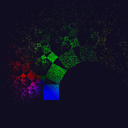
Browser renderer 1.0 
Chaotica
The original flame fractal paper mentions that there is no correct number of iterations. Generally, the following maxim holds true: the more the merrier. For educational purposes, I slowed down the iteration speed and rendered each and every step individually. This way you can see how the Chaos game is played out. Once you understand the concept you of course want to speed things up. One of the biggest bottlenecks is rendering pixels at each step. The trade-off is between being able to precisely see what’s being rendered and speed. We generally don’t care about the former as much as by the maxim more iterations usually lead to better renders. But, we’d still like to see some progress. This allows users to cut the rendering process short if the intermediate render is not up to standard. For now, let’s update the image every 100.000 iterations. We can now massively increase the total number of iterations or even let the image render indefinitely shifting the problem to patience. You can experience the trade-off here (normally I’d have the implementation here in the article, but WordPress won’t let me for some reason).
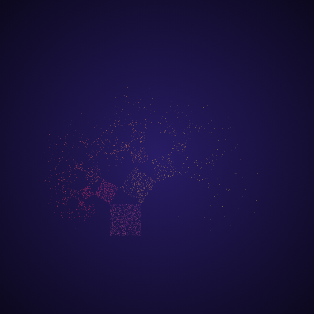
10K 
1M 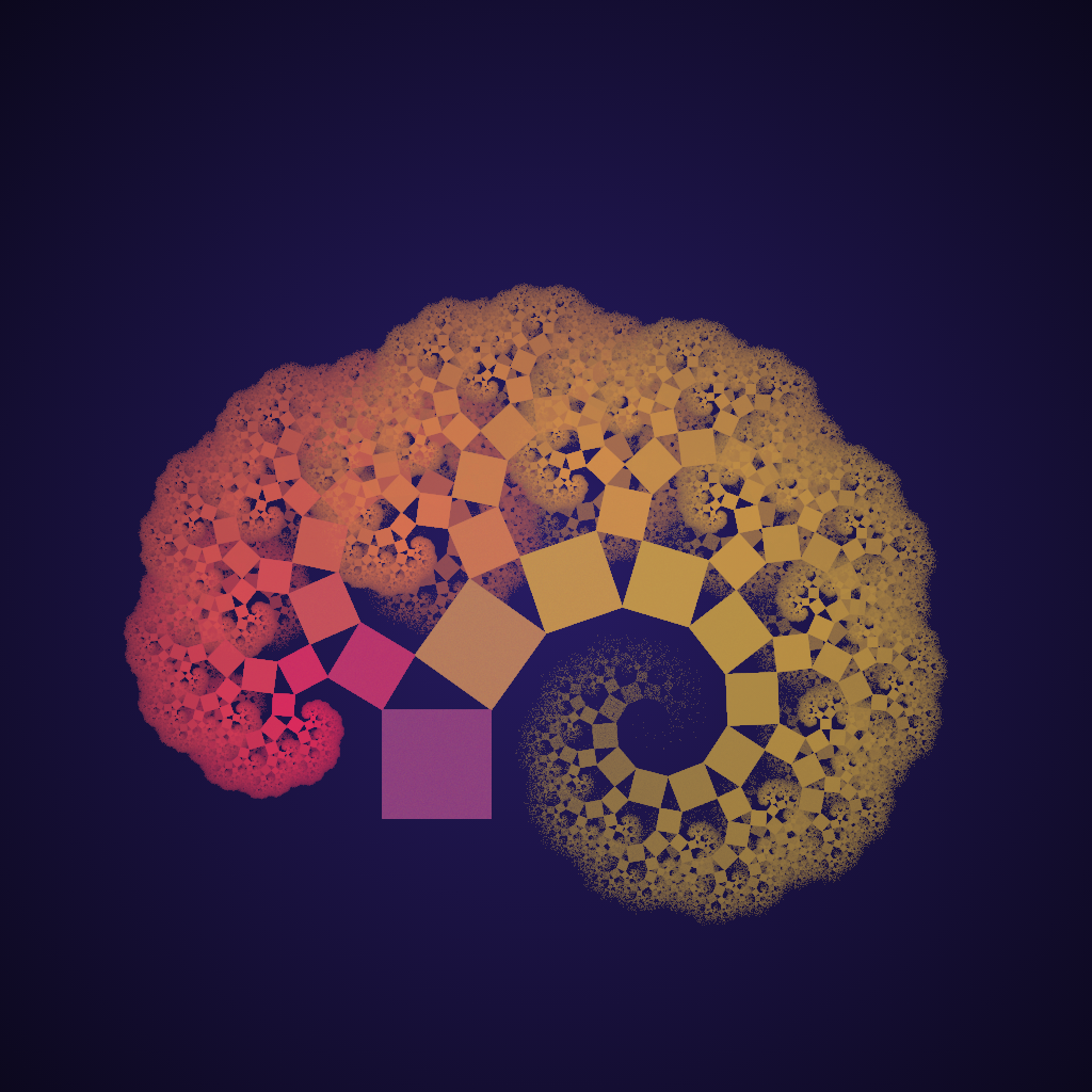
1B
The colours in previous images were fixed per pixel coordinates. Whether a pixel is coloured after function x or y doesn’t affect its appearance. By introducing a colour for each function in the system and changing the pixel colour with a function that uses this colour we can change this. Whenever a function is chosen at random, its associated colour is also chosen. We want a pixel to reflect the path of colours it has traversed. One way of doing this is by taking the average between the current colour and the chosen colour. The current colour factor experiences logarithmic decay over time, until it is visited again.
![\[c_{current}=\frac{1}{2}(c_{current} + c_{chosen})\]](https://matigekunstintelligentie.com/wp-content/ql-cache/quicklatex.com-dc67afbe11cf26db2fdd955c64db293b_l3.png "Rendered by QuickLaTeX.com")
Some areas of an IFS are visited more often than others. It would be nice if the frequency of visitation was reflected in the image. The first step is recording the frequency a pixel is reached in a buffer. You’ll also need to record the maximum frequency encountered over all pixels. You could then use the frequency divided by the maximum frequency to calculate the alpha channel of a pixel. More visited pixels then become more opaque. The issue with this technique is that certain areas are visited more than others. Looking back at the images from the first paragraph we see that the root of the tree is filled in nicely at a low number of iterations. The result of determining the alpha channel this way is that most parts of the tree would barely be visible. Applying a function that initially grows fast for low values and slow for large values would solve this problem. Taking the base 2 log of the value is a good choice.
After all these improvements the details may still be lost in darkness. To fix this a gamma correction should be applied to the alpha channel. A small gamma under 1.0 makes the image’s dark regions even darker. A gamma above 1.0 makes the image’s dark regions brighter. The gamma correction is done after rendering.
![\[\alpha=\alpha^{\frac{1}{\gamma}}\]](https://matigekunstintelligentie.com/wp-content/ql-cache/quicklatex.com-c0a1b0932666f0e344adce656b0a5d7e_l3.png "Rendered by QuickLaTeX.com")
There’s one more point left. Anti-aliasing. If you zoom in on the image you’ll see these jagged lines that should be straight. This is called aliasing and it can be fixed. This topic, however, deserves an article on its own.